this semester has been completely crazy for me, and i anticipate that this madness will only worsen over the next couple of months. of course, because of this crazy schedule, my brain started to revolt by growing a doubt inside me on how much i trust gradient descent. crazy, right? yes. i then succumbed to this temptation and looked for some simple example to test my trust in gradient descent. yes, i know that i should never doubt our lord Gradient Descent, but my belief is simply too weak.
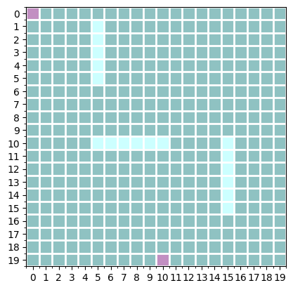
so, i decided to use gradient descent for simple trajectory planning given a 2D map. for instance, the following map is a sample map i decided to use for this exercise. the starting position is (0,0), and the goal position is (19,10). the sky blue blocks denote obstacles (or walls). the goal is to find a reasonable trajectory from the starting position to the goal position while avoiding the obstacles. in order to make the problem simpler (thereby my life simpler,) i assume the whole map is available. furthermore, we assume that each position in the map is discrete, i.e., represented as a tuple of integers, which makes it slightly tricky to use gradient descent.
the obstacle map is represented as
\[
m_o(i,j) = \begin{cases}
1,& \text{ if there is an obstacle at }(i,j) \\
0,& \text{ otherwise}
\end{cases}
\]
the goal position is simply represented as $(x_g, y_g)$.
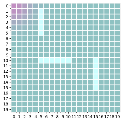
since the goal is to use gradient descent, we need to think about how to smooth the current position of a bot on the map, which allows us to compute the gradient of the loss function w.r.t. its current position. let $(x,y)$ be the current position of the bot. we then construct a _soft_ map showing the bot’s current position by setting the value of each coordinate $(i,j)$ as
\[
m_c(i,j) \propto \exp(-\frac{(x-i)^2 + (y-j)^2}{\beta}).
\]
we normalize $m_c(i,j)$ to sum to one. $\beta$ controls the smoothness of this map, and also tells us about our confidence in the bot’s position. this formulation allows us to compute the gradient of $m_c$ with respect to $(x,y)$. here’s a sample of the soft map of the current position $(0,0)$ with $\beta=0.1$ (for the purpose of better visualization):
now we initialize the trajectory of a fixed number of steps randomly by
\[
\mathcal{T}_x(t) \sim \mathcal{U}(0, x_{\max})\quad\text{and}\quad
\mathcal{T}_y(t) \sim \mathcal{U}(0, y_{\max}).
\]
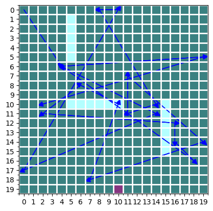
an example of a random trajectory is shown here. not really great, is it? it’s all over the place, overlaps with the obstacles and also each transition is unrealistic for our bot to take.
how would we know whether the bot is too close to the obstacle? the soft map formula above turned out to be extremely handy in this case, as all we need to do is to compute the expected obstacleness of the map given the soft map of the bot’s current position, as in
\[
s(m_c) = \sum_{i,j} m_c(i,j) \times m_o(i,j).
\]
if the bot is near the obstacle, this score would be high. if the bot is far away from any obstacle, the score would converge toward $0$.
now, we need to design a loss function to be minimized by gradient descent with respect to the bot’s positions in the trajectory. more specifically, the loss function needs at least the four terms.
- the distance of the final position in the trajectory to the goal position $L_1(\mathcal{T}) = \| \mathcal{T}_{x,y}(T) – [x_g, y_g] \|$.
- the amount of collision with the obstacle $L_2(\mathcal{T}) = \sum_{t=1}^T s(m_{\mathcal{T}_{x,y}}(t))$.
- the distance of the initial position of the trajectory to the starting position $L_3(\mathcal{T}) = \| \mathcal{T}_{x,y}(T) – [x_s, y_s] \|$.
- the smoothness of the trajectory $L_4(\mathcal{T}) = \sum_{t=1}^{T-1} \| \mathcal{T}_{x,y}(t) – \mathcal{T}_{x,y}(t+1) \|$.
the first one is trivially understandable, since we want the planned trajectory to end up near the goal. the second one is also understandable, as we want to minimize the chance of colliding into the obstracles/walls in the planned trajectory. the third term is there to ensure that the trajectory starts from where the bot was placed.
the final one is there to ensure that the transition from one position to the next position within the trajectory is small enough so that our bot’s actuator can execute this transition without too much trouble. Without this term, the trajectory could very well simply jump from the starting point to the goal point in one step and call it a day.
the final loss w.r.t. the trajectory is then the weighted sum of these loss functions:
\[
L(\mathcal{T}) = \sum_{k=1}^4 \omega_k L_k(\mathcal{T}).
\]
Because $L$ is differentiable w.r.t. all positions in $\mathcal{T}$, you can now use your favourite optimization algorithm (in my case, i will stick to naive gradient descent here). you can also let your favourite software package compute the gradient $\nabla_{\mathcal{T}} (L)$ automatically for you (in my case, i use PyTorch.)
one final step we need after performing gradient descent is to discretize each estimated point in the final trajectory, as we assumed that the map is given to us as a discrete grid. in this particular case, i simply round each coordinate to the nearest integer. that is, for all $t=1,\ldots,T$,
\[
\mathcal{T}_x(t) \leftarrow \mathrm{round}(\mathcal{T}_x(t))
\quad\text{ and }\quad
\mathcal{T}_y(t) \leftarrow \mathrm{round}(\mathcal{T}_y(t))
\]
in this particular example, i’ve set the learning rate to $0.1$ and ran $1,000$ steps of gradient descent (probably unnecessarily many, though) on a trajectory of length 20. this results in the following optimized trajectory after rounding:
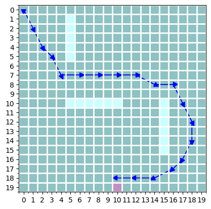
it slightly missed the goal by one, but the trajectory looks pretty reasonable. each transition is more or less about 2-3 blocks long, and the final point is within 1 block away from the goal. it also avoids all three walls perfectly.
at the end of the day, gradient descent has stood yet another test, and i must repent my sin of doubting the almighty gradient descent. it even works well on planning on a discretized 2d grid, although it was probably too simple a map for any algorithm to fail. indeed, i recall that one of the homework assignments from the course on Probabilistic Robotics by Prof. Kee Eung Kim at KAIST long time ago was to build a planner in almost exactly the same environment however using dynamic programming.
what can we do further if we want to test our trust in gradient descent further? we can introduce a potentially noisy differentiable model of the bot’s actuation and try to optimize the trajectory of not positions but controls. we can also perform this planning repeatedly as the bot makes progress toward the goal to make it more realistic. finally, we can imagine extending it to a partially-observed environment, where we also run gradient descent based inference on missing parts of the map. many interesting problems … that are not new but have been studied extensively in the fields of robotics, control and machine learning … 🙂
you can find the code at the following Github repo. it includes both the main code and the notebook to reproduce all the figures above:
https://github.com/kyunghyuncho/map_plan_backprop/
and … i heard i must disclose these days what i have used to do any research/development. hence, here you go: i’ve used Visual Studio Code with Github CoPilot.