this post continues from the previous post <Gradient-based trajecotry planning>, because i became even busier. in fact, i should work on my presentation slide for my talk at the University of Washington tomorrow (sorry, Yejin and Noah!), and probably because of that, i decided to push it a bit further.
the main assumption i made in the previous slide was that our bot has access to the entire map. this is a huge assumption that does not often hold in practice. instead, i decided to restrict the visibility of our bot. it will be able to see the obstacles in its neighbourhood. furthermore, this visibility will be noise. this noisy observation is implemented as:
\[
\tilde{m}_o(i,j) = \min(\max(m_c(i,j) m_o(i,j) + \epsilon_{i,j}, 0), 1),
\]
where $m_c(i,j)$ and $m_o(i,j)$ are the soft map of the current position of the bot and the true obstacle map, respectively. they were defined in the previous post. $\epsilon_{i,j}$ is the observational noise.
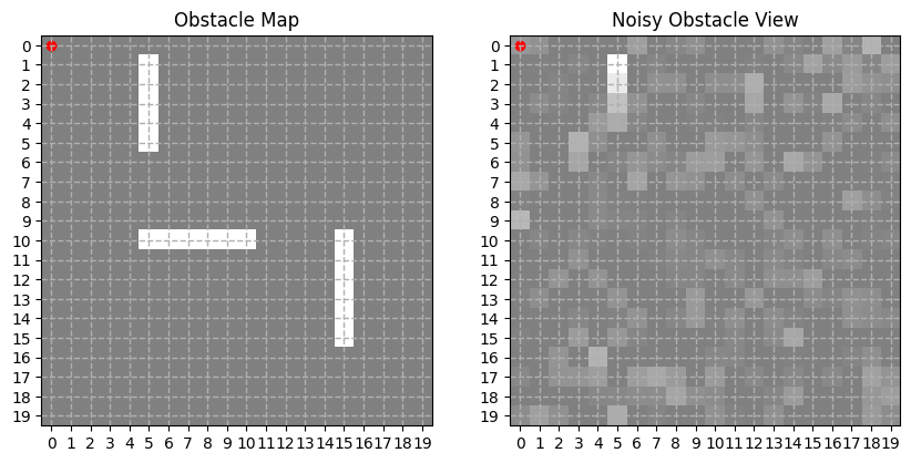
as an example, when the true map with the walls was like on the left panel, the bot, which is situated in the top left corner, would see the map on the right panel, below. this is with Gaussian noise of mean $0$ and standard deviation $0.001$. so, it can get a glimpse of the wall, but there’s quite a bit of noise.
for estimating the true map based on successive noisy observations, we will again rely on Our Lord gradient descent. although there must be a better loss function, i got lazy and decided to use the simplest possible version here:
\[
l_{\mathrm{map}}(\hat{m}_o, \tilde{m}_o) =
\sum_{i,j} | m_c(i,j) \cdot \mathrm{sigmoid}(\hat{m}_o(i,j)) – \tilde{m}_o(i,j) |,
\]
where $\hat{m}_o(i,j)$ is a logit. why do i estimate the logit instead of the actual $[0,1]$ value of each position? because i am a deep learner.
because the bot is restless and moves around, it’s not easy to interpret what it means to minimize this loss function. if we assume the bot is in a fixed location, we can however interpret this as estimating the underlying map from repeated observations by assuming that noise will cancel out across those observations. this is a good interpretation, but also reveals a weakness of this approach. that is, it will not work well with biased noise. i won’t address this here, but this shouldn’t be too difficult to address as long as we know the noise model (but how!?)
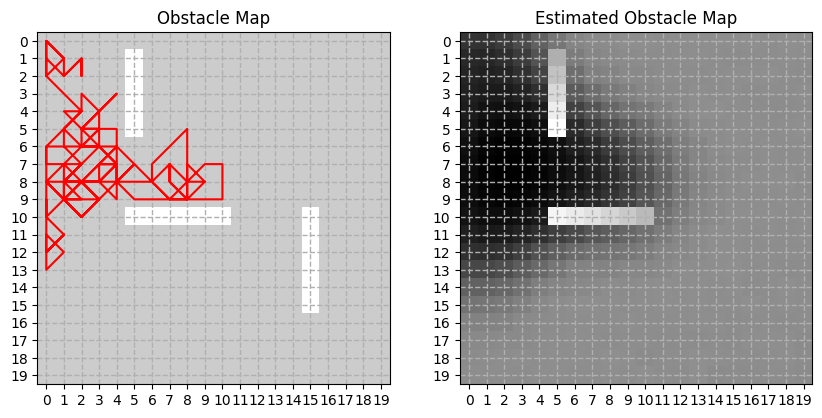
so, how well does it work? i’ve implemented as a very simple random-walk bot and let it walk over the same map from the previous post. while taking the stroll, the bot kept updating its internal view of the map. as you can see below, the bot is able to figure out where walls are, when those walls are near where it has been.
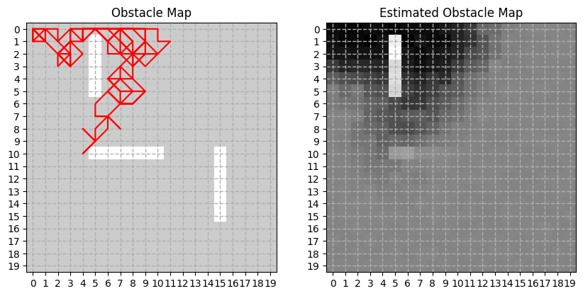
when the level of noise is higher ($0.01$), the estimated map is indeed noisier:
you can check the mapping code at https://github.com/kyunghyuncho/map_plan_backprop/blob/main/test_mapping.ipynb.
now we have two components we need in order to endow our bot an ability to navigate toward a given goal location when it does not have access to the map. given the current position of the bot and the goal position, the bot can repeat the following steps to reach the goal position in an unknown environment:
- observe the environment and update its map estimate using several gradient descent updates.
- plan the trajectory toward the goal given the estimated map so far using several gradient descent updates.
- take a small step toward the first position in the trajectory, that is different from the current position.
the size of the small step in (3) above is determined based on the actuator of the bot, and we can assume for now that it can move to any positions within up to 3 steps away in each axis. of course, the bot cannot move out of the map nor run over the wall. it will simply stop when it hits the wall, just like your Roomba at home does.
first, we want to know if this scheme works when there is no observation noise. although there is no noise, observation is not full, in the sense that it has only limited visibility into the neighbourhood of the current position. the bot is taking 20 Adam updates for both updating the map estimate and producting the trajectory after each move in this case. i ran it up to 500 steps but allowed the bot to terminate when it is within distance 2 from the goal position.
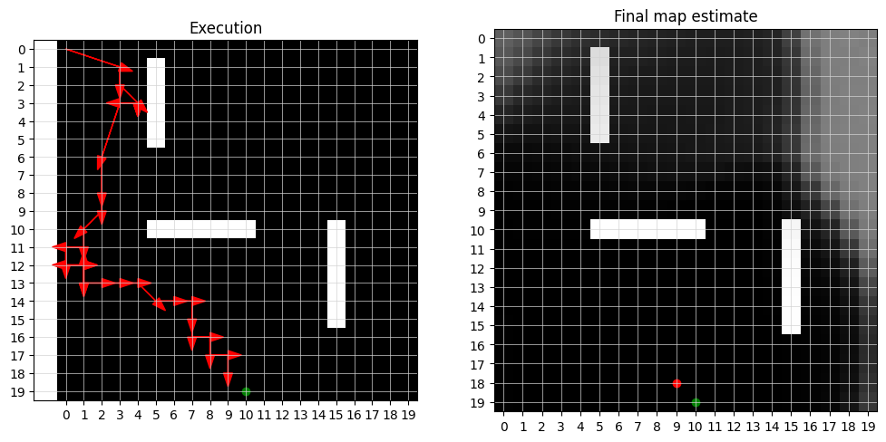
as you can see here, it works pretty much perfectly. near the end of the execution, the bot has a good estimate of the entire map, except for the top right corner which was very far away from the bot’s trajectory. because there was no noise, we see very crisp estimates of the walls.
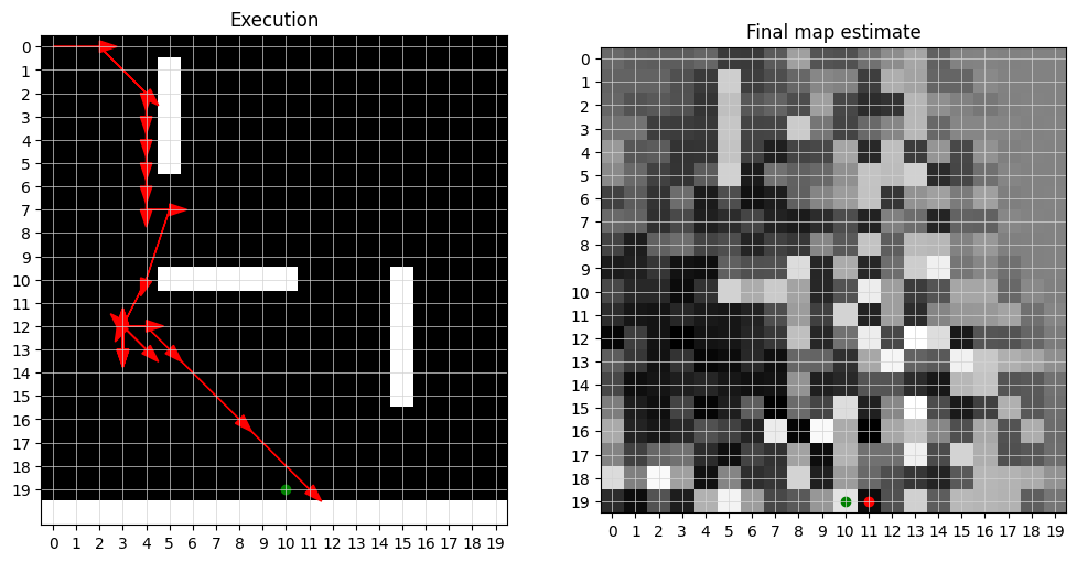
when the noise level increases to $0.01$, we start to observe that the bot’s estimate of the map is quite rough, as below. near the bot’s trajectory, we can notice some of the true walls, but even slight further away, the bot has pretty much no idea how the whole environment looks like. the third wall (the bottom right one) simply doesn’t show up at all in the bot’s map estimate. Nevertheless, the bot successfully reached the goal, since the local estimate is all that matters in this case, just like how actor-critic algorithms in reinforcement learning do not often require us to have a global critic but only a local critic (and often just a linear approximation to it.)
you can reproduce the figures above and play around with our first autonomous bot almost entirely based on gradient descent at https://github.com/kyunghyuncho/map_plan_backprop/blob/main/test_move.ipynb.
although i wrote it as if everything can be done as gradient descent, that’s not true, as it becomes eventually necessary to discretize the outcome of gradient descent in order to interact with the world (i.e. the 2-D grid in our case.) for this, i had to add in a number of heuristics here and there to avoid various degenerate cases such as gradient descent taking a zero-discrete step. you can check all these heuristics (though, there are only a few) at https://github.com/kyunghyuncho/map_plan_backprop.
of course, you can now imagine what the next step would be. the next step should be for us to grant our bot an ability to localize its own location, which was assumed to be given so far. once we are done with localization, we would end up with a full gradient-based autonomous bot that can simultaneously localize, map and navigate in an unknown environment. this will however have to wait until my next decompression coding (what a beautiful phrase, Jakob!)
and, if you’re interested in building autonomous robots based on machine learning, don’t forget to check out <Probabilistic Robotics> by Sebastian Thrun.