[UPDATE: Feb 8 2025] my amazing colleague Max Shen noticed a sign mistake in my derivation of the partial derivative of the log-harmonic function below.
i taught my first full-semester course on <Natural Language Processing with Distributed Representation> in fall 2015 (whoa, a decade ago!) you can find the lecture note from this course at https://arxiv.org/abs/1511.07916.
in one of the lectures, David Rosenberg, who was teaching machine learning at NYU back then and had absolutely no reason other than kindness to sit in at my course, asked why we use softmax and whether this is the only way to turn unnormalized real values into a categorial distribution. it was right after i introduce softmax to the class simply as a way to transform a real vector to satisfy (1) non-negativity and (2) normalization: $\frac{\exp(a_i)}{\sum_j \exp(a_j)}$. and, sadly, i was totally stuck, babbled a bit and moved on.
although i could not pull out the answer immediately on the spot (you gotta give my 10-years-younger me a bit of a slack; it was my first full course,) there are a number of reasons why we like softmax. the first reason i often bring up is the principle of maximum entropy, which is how i just introduced softmax to the students at <Machine Learning> this semester. simply put, we can derive softmax by maximizing a weighted sum of the expected negative energy and the shannon entropy. the latter term (the entropy) corresponds to the maximum entropy principle. this is just very nice, and can be extended to work with different inductive biases, such as sparsity (check out this beautiful work https://arxiv.org/abs/1602.02068 by Andre Martins and Ramon Astudillo, and an extensive follow-up studies summarized in this beautiful talk by Andre; https://andre-martins.github.io/docs/taln2021.pdf)
the second reason, which is my actual favourite, is that the learning signal we get from softmax is extremely intuitive and interpretable. the partial derivative of log softmax w.r.t. each input real value can be written down as
$$
\frac{\partial }{\partial a_k} \log \frac{\exp(a_i)}{\sum_j \exp(a_j)} = \mathbb{I}(k=i) – \frac{\exp(a_k)}{\sum_j \exp(a_j)},
$$
where $i$ is the target class.
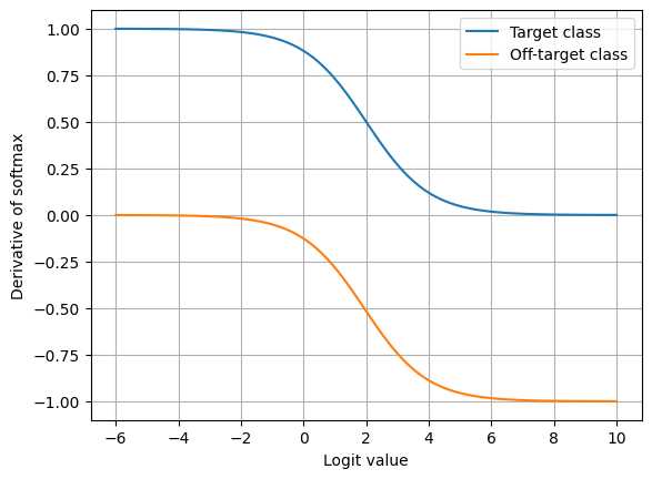
why is this intuitive and interpretable? this gradient says that this categorical distribution defined using softmax should gradually match the extreme categorical distribution where the entire probability mass is concentrated on the target class (correct answer.) as it gets closer and closer to this extreme distribution, that is one of the vertices of the simplex, the gradient norm shrinks and eventually converges toward zero. we can easily see that from the plot below. as learning progresses, the gradient norm shrinks toward 0.
during the past few days, there was a paper posted on arXiv that claims that so-called harmonic formulation is better than softmax, in terms of training a neural net.* i kinda stopped reading this paper when i noticed that they “trained the MLP models for 7000 epochs and the transformers for 10000 epochs. For all four models, we used the AdamW optimizer with a learning rate of 2×10⁻³, a weight decay of 10−2, and an L2 regularization on the embeddings with strength 0.01.” it’s really impossible to choose an arbitrary hyperparameter configuration and empirically compare different learning algorithms.
anyhow, i digressed. instead of further reading this paper, i just wanted to see what this harmonic formulation was. this turned out to be
$$
p(i) = \frac{|a_i|^{-n}}{\sum_j |a_j|^{-n}},
$$
where $n \geq 1$ is a hyperparameter. this is precisely what David Rosenberg asked me nearly 10 years ago; “why not using squares instead of exponentials?” (paraphrased from my memory)
without thinking much about it, it is easy to see that this formulation is not really friendly to gradient based optimization. let’s look at the partial derivative of the log-harmonic, similarly to that of log-softmax above,
$$
\frac{\partial }{\partial a_k } \log \frac{|a_i|^{-n}}{\sum_j |a_j|^{-n}} =
-\mathbb{I}(i=k) \frac{n~\mathrm{sign}(a_i)}{|a_i|}
+ n~\mathrm{sign}(a_k) \frac{|a_k|^{-n-1}}{\sum_j |a_j|^{-n}}.
$$
just like before, let’s consider the target and off-target classes separately. first, the target class:
$$
-\frac{n~\mathrm{sign}(a_i)}{|a_i|}\underbrace{ \left( 1 – q(a_i) \right)}_{=\mathrm{(a)} \geq 0},
$$
where $q(a_i)$ is the probability of $i$ under the harmonic formulation. the direction (sign) of the derivative is entirely determined by the sign of $a_i$, and it points to the opposite direction. that is, it always drives $a_i$ toward $0$.
it’s the opposite with the off-target class:
$$
\frac{n~\mathrm{sign}(a_j)}{|a_j|}\underbrace{ \left( q(a_j) \right)}_{=\mathrm{(b)}>0},
$$
depending on which side of the origin $a_i$ is, it is driven toward the negative extreme (either $\infty$ or $-\infty$.) there is a degeneracy at the origin, since this decision (whether to go to $\infty$ or $-\infty$) cannot be broken on its own.
there are two things that make me feel somewhat uncomfortable. first, the minimum for the target class is singular, in that it will likely oscillate, unlike softmax above. second, the magnitude of the derivative w.r.t. the off-target logit is extremely large near the origin (in fact, it diverges) and converges to 0 rapidly as it deviates away from the origin. the magnitude in fact is essentially zero already by $-1$ and $1$, and there won’t be much of a learning signal (i.e. vanishing gradient) unless things were initialized very carefully. one big step early on (when $|a_k| \approx 0$) will result in zero learning signal immediately. these observations are summarized in the following plot:
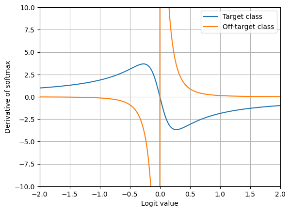
why does it exhibit such an extreme behaviour at the origin? it’s because of the symmetry of the absolute function, $|a_k|$. it’s perfectly fine to either decrease or increase $a_k$ to make the probability associated with $k$ to decrease. the only way for the probability to increase is of $a_k$ to approach $0$ from either side of the origin. such a symmetry makes learning very challenging.
but then … does it really matter? as i told the students at my course last week, learning isn’t optimization, and perhaps it really doesn’t matter as long as we can make little progress at a time with iterative optimization. especially with powerful tools like reverse-mode autodiff, Adam and more, we perhaps don’t have to worry about the gradient of the loss too much.
anyhow, to cap this post, i have to wonder if there is any way to save this approach. one way i can think of is to introduce a margin $m$, such as
$$
| \max(0, a_k – m) |^{-n},
$$
and start sounding like Yann LeCun. perhaps another way is to simply give up and enjoy Friday evening with the happy hour drink at the office.
oh, you can reproduce the plots above at https://github.com/kyunghyuncho/softmax-forever/blob/main/softmax_forever.ipynb.
(*) i am not going to point to that paper, since i am worried this post may come off as criticizing the student authors of the paper (though, i am certainly ready to criticize the supervising faculty ;))